Introduction to Jupyter Notebook (Part 1)
Contents
Introduction to Jupyter Notebook (Part 1)#
gfbio Winterschool 2022, Sophie Wolf
Jupyter refers to Julia, Python and R
Jupyter Notebook (formerly IPython Notebooks) is a web-based open-source interactive computational environment.
A notbook contains a list of input and output cells, which can contain:
# code
1+1
2
Text formatted with Markdown
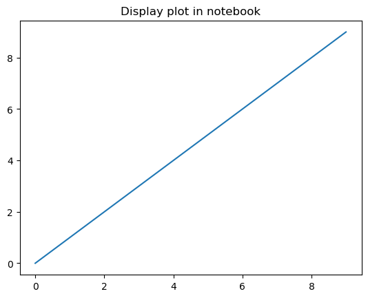
import matplotlib.pyplot as plt

plt.plot(range(10))
plt.title('Display plot in notebook')
plt.show()

Creating a new notebook#
Kernels
We will be using Python 3 and R kernels.
First orientation#
user interface tour
command mode and edit mode
keyboard shortcuts
print("Winterschool 2022")
Winterschool 2022
title = "Winterschool 2022"
title
'Winterschool 2022'
"Winterschool 2022"
'Winterschool 2022'
Supress output using ;
"Winterschool 2023";
🤖 Try it!#
Take a few minutes to explore the keyboard shortcuts.
Ordering of executions#
Be mindful: You can execute Jupyter cells in any order. The execution order is displayed as numbers to the left of each code cell.
species = "Nepeta cataria"
species
'Theobroma cacao'
species = "Theobroma cacao"
A few remarks on Markdown#
Markdown is a simple markup language for creating formatted text using a plain-text editor.
Some functions#
italics
bold
code block here
You can create things like this nice table:
Some traits in TRY database |
ID |
Unit |
|---|---|---|
Leaf area (in case of compound leaves: leaflet, undefined if petiole is in- or excluded) |
3113 |
mm2 |
Leaf area per leaf dry mass (specific leaf area, SLA or 1/LMA): undefined if petiole is in- or excluded) |
3117 |
m2/kg |
Stem specific density (SSD) or wood density (stem dry mass per stem fresh volume) |
4 |
g/cm3 |
Leaf carbon (C) content per leaf dry mass |
13 |
mg/g |
Leaf nitrogen (N) content per leaf dry mass |
14 |
mg/g |
Leaf phosphorus (P) content per leaf dry mass |
15 |
mg/g |
Plant height vegetative |
3106 |
m |
Or insert an image from your local machine or url.

This image is a citizen science observation from the project iNaturalist.
Line magic and cell magic#
Jupyter has a whole library of so-called line or cell magic. These allow you to switch to other programming languages within on single Jupyter notebook.
bash command#
To access the terminal simply use an ! before your bash command.
!pwd
/Users/sophiewolf/Documents/GitHub/Jupyter_Workshop_Winterschool_2022
For example, you could use it to install a new package:
!pip install tqdm
There are many in-built options for line and cell magics. They always start with:
%for line magic%%for cell magic
To list all the built-in available magic commands type the following:
%lsmagic
Available line magics:
%alias  %alias_magic  %autoawait  %autocall  %automagic  %autosave  %bookmark  %cat  %cd  %clear  %colors  %conda  %config  %connect_info  %cp  %debug  %dhist  %dirs  %doctest_mode  %ed  %edit  %env  %gui  %hist  %history  %killbgscripts  %ldir  %less  %lf  %lk  %ll  %load  %load_ext  %loadpy  %logoff  %logon  %logstart  %logstate  %logstop  %ls  %lsmagic  %lx  %macro  %magic  %man  %matplotlib  %mkdir  %more  %mv  %notebook  %page  %pastebin  %pdb  %pdef  %pdoc  %pfile  %pinfo  %pinfo2  %pip  %popd  %pprint  %precision  %prun  %psearch  %psource  %pushd  %pwd  %pycat  %pylab  %qtconsole  %quickref  %recall  %rehashx  %reload_ext  %rep  %rerun  %reset  %reset_selective  %rm  %rmdir  %run  %save  %sc  %set_env  %store  %sx  %system  %tb  %time  %timeit  %unalias  %unload_ext  %who  %who_ls  %whos  %xdel  %xmode

Available cell magics:
%%!  %%HTML  %%SVG  %%bash  %%capture  %%debug  %%file  %%html  %%javascript  %%js  %%latex  %%markdown  %%perl  %%prun  %%pypy  %%python  %%python2  %%python3  %%ruby  %%script  %%sh  %%svg  %%sx  %%system  %%time  %%timeit  %%writefile

Automagic is ON, % prefix IS NOT needed for line magics.
Line magic refers only to the one line. So all code before and after this line within the same cell will be interpreted as the kernel language, in our case Python 3. There are many bash line magic commands, such as %ls or %pwd.
%ls

print("Hi! I'm Python code.")
!echo "And I'm bash script."
Data/
Figures/
README.md
Winterschool_2022_Additional_Materials.ipynb
Winterschool_2022_Jupyter_Data_Analysis.ipynb
Winterschool_2022_Jupyter_Introduction.ipynb
Winterschool_2022_R_Kernel.ipynb
requirements.txt
Hi! I'm Python code.
And I'm bash script.
Cell magic applies to the whole cell, so all code will be interpreted in reference to the magic command. As a result, the following command will generate an error. Cell magic must always be placed at the top of the cell.
%%bash

ls
echo "Hi! I'm bash script."
print("And I'm Python code.")
Data
Figures
README.md
Winterschool_2022_Additional_Materials.ipynb
Winterschool_2022_Jupyter_Data_Analysis.ipynb
Winterschool_2022_Jupyter_Introduction.ipynb
Winterschool_2022_R_Kernel.ipynb
requirements.txt
Hi! I'm bash script.
bash: line 4: syntax error near unexpected token `"And I'm Python code."'
bash: line 4: `print("And I'm Python code.")'
---------------------------------------------------------------------------
CalledProcessError                        Traceback (most recent call last)
Cell In [15], line 1
----> 1 get_ipython().run_cell_magic('bash', '', '\nls\necho "Hi! I\'m bash script."\nprint("And I\'m Python code.")\n')

File ~/miniforge3/envs/winterschool/lib/python3.8/site-packages/IPython/core/interactiveshell.py:2417, in InteractiveShell.run_cell_magic(self, magic_name, line, cell)
   2415 with self.builtin_trap:
   2416     args = (magic_arg_s, cell)
-> 2417     result = fn(*args, **kwargs)
   2418 return result

File ~/miniforge3/envs/winterschool/lib/python3.8/site-packages/IPython/core/magics/script.py:153, in ScriptMagics._make_script_magic.<locals>.named_script_magic(line, cell)
    151 else:
    152     line = script
--> 153 return self.shebang(line, cell)

File ~/miniforge3/envs/winterschool/lib/python3.8/site-packages/IPython/core/magics/script.py:305, in ScriptMagics.shebang(self, line, cell)
    300 if args.raise_error and p.returncode != 0:
    301     # If we get here and p.returncode is still None, we must have
    302     # killed it but not yet seen its return code. We don't wait for it,
    303     # in case it's stuck in uninterruptible sleep. -9 = SIGKILL
    304     rc = p.returncode or -9
--> 305     raise CalledProcessError(rc, cell)

CalledProcessError: Command 'b'\nls\necho "Hi! I\'m bash script."\nprint("And I\'m Python code.")\n'' returned non-zero exit status 2.
Since Jupyter cells can be executed in any order, you might need to check your notebooks variables. The following commands can be very useful:
# current variable names

%who
plt species title
# current variables, incl. type and data

%whos
Variable   Type      Data/Info
------------------------------
plt        module    <module 'matplotlib.pyplo<...>es/matplotlib/pyplot.py'>
species    str       Theobroma cacao
title      str       Winterschool 2022
Remove a specific variable from environment:
%reset_selective species
Once deleted, variables cannot be recovered. Proceed (y/[n])? y
Remove all variables from environment:
%reset
Once deleted, variables cannot be recovered. Proceed (y/[n])? n
Nothing done.
How to embed a video:
%%HTML
<iframe width="700" height="500"
    src="https://www.youtube.com/embed/HW29067qVWk"
    frameborder="0"
    allowfullscreen></iframe>
🤖 Try it!#
Take a few minutes to play around with the line and cell magic commands. Create some variables and remove them again.
Visualize plots#
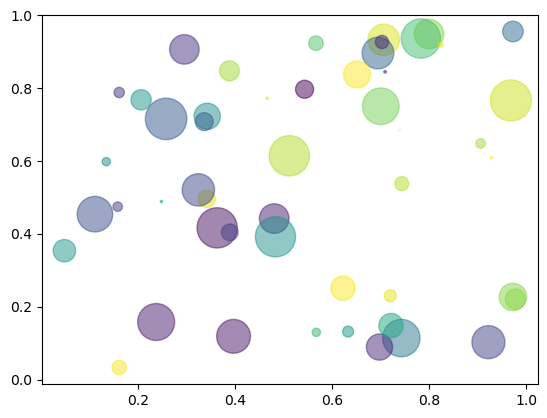
# Example from matplotlib documentation

import numpy as np # arrays and such
import matplotlib.pyplot as plt # plotting

# Fixing random state for reproducibility
np.random.seed(19680801)


N = 50
x = np.random.rand(N)
y = np.random.rand(N)
colors = np.random.rand(N)
area = (30 * np.random.rand(N))**2  # 0 to 15 point radii

plt.scatter(x, y, s=area, c=colors, alpha=0.5)
plt.show()

Execution time#
If you want to test the speed of your code, the %%time magic can be very useful.
%%time
plt.scatter(x, y, s=area, c=colors, alpha=0.5)
plt.show()

CPU times: user 57.1 ms, sys: 4.01 ms, total: 61.1 ms
Wall time: 59.2 ms
Look up documentation#
If you want to check the documentation of the function you want to use, simply click inside the function and press Shift+Tab. Or, if that doesn’t help, look it up using your favorite search engine!
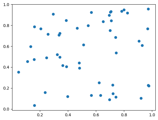
plt.scatter(x, y);

Dataframes#
import pandas as pd #handles dataframes in Python
import numpy as np #arrays and such in Python

# create sample dataframe

df = pd.DataFrame(np.random.randn(100,5), columns=["A","B","C","D","E"])
df
| A | B | C | D | E | |
|---|---|---|---|---|---|
| 0 | 0.835275 | 0.181993 | 1.232291 | -0.996842 | -0.804238 |
| 1 | 1.833230 | 0.084046 | -0.466226 | -0.458791 | -0.623695 |
| 2 | 0.645133 | -1.851581 | 0.843342 | 1.093867 | 0.456576 |
| 3 | 0.273131 | -1.916821 | 0.162999 | 0.920437 | -0.667275 |
| 4 | -0.046662 | -0.613771 | -0.374934 | 0.516941 | 0.538914 |
| ... | ... | ... | ... | ... | ... |
| 95 | -1.207959 | -0.517363 | 0.597141 | 0.588914 | -0.872500 |
| 96 | 0.691405 | 0.009598 | -0.211532 | -0.821576 | 0.920173 |
| 97 | -1.025475 | 0.269079 | 1.641999 | -1.113975 | -0.174968 |
| 98 | -0.787913 | -0.093945 | -0.791022 | -1.639523 | -1.884071 |
| 99 | -0.512947 | 0.432264 | -1.149004 | 0.731894 | -1.413364 |
100 rows × 5 columns
# display only the first 5 rows
df.head(5)
| A | B | C | D | E | |
|---|---|---|---|---|---|
| 0 | 0.835275 | 0.181993 | 1.232291 | -0.996842 | -0.804238 |
| 1 | 1.833230 | 0.084046 | -0.466226 | -0.458791 | -0.623695 |
| 2 | 0.645133 | -1.851581 | 0.843342 | 1.093867 | 0.456576 |
| 3 | 0.273131 | -1.916821 | 0.162999 | 0.920437 | -0.667275 |
| 4 | -0.046662 | -0.613771 | -0.374934 | 0.516941 | 0.538914 |
🤖 Try it!#
Use the scatter plot function above together with data from the sample dataframe df. Look up the plt.scatter() documentation to add features to your plot.
# play around with scatter plot function
Using R within a Python Juypter notebook#
R Magic#
To use R within a Python Juypter notebook, which was intitiated using a Python kernel, we need so-called R magic.
# enables the %%R magic, needs to be installed and then activated only once per Notebook
%load_ext rpy2.ipython
As we’ve seen before, % denotes line magic, while %% denotes cell magic. R magic uses the same syntax.
%R x <- c(1, 2, 3)

x
array([0.7003673 , 0.74275081, 0.70928001, 0.56674552, 0.97778533,
       0.70633485, 0.24791576, 0.15788335, 0.69769852, 0.71995667,
       0.25774443, 0.34154678, 0.96876117, 0.6945071 , 0.46638326,
       0.7028127 , 0.51178587, 0.92874137, 0.7397693 , 0.62243903,
       0.65154547, 0.39680761, 0.54323939, 0.79989953, 0.72154473,
       0.29536398, 0.16094588, 0.20612551, 0.13432539, 0.48060502,
       0.34252181, 0.36296929, 0.97291764, 0.11094361, 0.38826409,
       0.78306588, 0.97289726, 0.48320961, 0.33642111, 0.56741904,
       0.04794151, 0.38893703, 0.90630365, 0.16101821, 0.74362113,
       0.63297416, 0.32418002, 0.92237653, 0.23722644, 0.82394557])
R variables can also be used across different cells, as long as you call R magic every time.
%R x
array([1., 2., 3.])
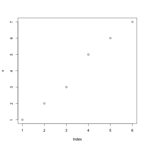
%%R

x <- append(x, c(5,6,7))
plot(x)

Move variables from Python environment to R, and vice versa#
%whos
Variable   Type         Data/Info
---------------------------------
N          int          50
area       ndarray      50: 50 elems, type `float64`, 400 bytes
colors     ndarray      50: 50 elems, type `float64`, 400 bytes
df         DataFrame               A         B   <...>n\n[100 rows x 5 columns]
np         module       <module 'numpy' from '/Us<...>kages/numpy/__init__.py'>
pd         module       <module 'pandas' from '/U<...>ages/pandas/__init__.py'>
plt        module       <module 'matplotlib.pyplo<...>es/matplotlib/pyplot.py'>
title      str          Winterschool 2022
x          ndarray      50: 50 elems, type `float64`, 400 bytes
y          ndarray      50: 50 elems, type `float64`, 400 bytes
%Rpush df
%R df
| A | B | C | D | E | |
|---|---|---|---|---|---|
| 0 | 0.835275 | 0.181993 | 1.232291 | -0.996842 | -0.804238 |
| 1 | 1.833230 | 0.084046 | -0.466226 | -0.458791 | -0.623695 |
| 2 | 0.645133 | -1.851581 | 0.843342 | 1.093867 | 0.456576 |
| 3 | 0.273131 | -1.916821 | 0.162999 | 0.920437 | -0.667275 |
| 4 | -0.046662 | -0.613771 | -0.374934 | 0.516941 | 0.538914 |
| ... | ... | ... | ... | ... | ... |
| 95 | -1.207959 | -0.517363 | 0.597141 | 0.588914 | -0.872500 |
| 96 | 0.691405 | 0.009598 | -0.211532 | -0.821576 | 0.920173 |
| 97 | -1.025475 | 0.269079 | 1.641999 | -1.113975 | -0.174968 |
| 98 | -0.787913 | -0.093945 | -0.791022 | -1.639523 | -1.884071 |
| 99 | -0.512947 | 0.432264 | -1.149004 | 0.731894 | -1.413364 |
100 rows × 5 columns
%%R

correlation <- cor(df$A, df$B)
correlation
[1] -0.04536287
correlation = %Rget correlation
correlation
array([-0.04536287])
Create a new notebook using an R kernel#
See file Winterschool_2022_R_Kernel.ipynb
Practical example with vegetation data#
# import required packages

import pandas as pd #for data frames
import numpy as np #
from matplotlib import pyplot as plt #for plotting
sPlotOpen#
sPlotOpen (Sabatini et al, 2021) is an open-access and environmentally and spatially balanced subset of the global sPlot vegetation plots data set v2.1 (Bruelheide et al, 2019).
For future reference, sPlotOpen Data is available at the iDiv Data Repository. For this study we used version 52, which you can download using the following link: https://idata.idiv.de/ddm/Data/ShowData/3474
The data is stored in various tab-separated files:
sPlotOpen_header(2).txt : contains information on each plot, such as coordinates, date, biome, country, etc.
sPlotOpen_DT(1).txt : contains information per plot and species with abundance and relative cover
sPlotOpen_CWM_CWV(1).txt : contains information on trait community weighted means and variances for each plot and 18 traits (ln-transformed)
For this example, we will look at the trait community weighted means.
cwm = pd.read_csv("Data/sPlotOpen_CWM_CWV(1).txt", sep= "\t")
View the first 5 rows of data frame. Note: All values are in natural logarithm.
cwm.head()
| PlotObservationID | TraitCoverage_cover | Species_richness | TraitCoverage_pa | LeafArea_CWM | StemDens_CWM | SLA_CWM | LeafC_perdrymass_CWM | LeafN_CWM | LeafP_CWM | ... | Seed_length_CWV | LDMC_CWV | LeafNperArea_CWV | LeafNPratio_CWV | Leaf_delta_15N_CWV | Seed_num_rep_unit_CWV | Leaffreshmass_CWV | Stem_cond_dens_CWV | Disp_unit_leng_CWV | Wood_vessel_length_CWV | |
|---|---|---|---|---|---|---|---|---|---|---|---|---|---|---|---|---|---|---|---|---|---|
| 0 | 16 | 0.277778 | 3 | 0.333333 | 3.678311 | -1.047293 | 2.890748 | 6.128157 | 2.873263 | 1.114036 | ... | NaN | NaN | NaN | NaN | NaN | NaN | NaN | NaN | NaN | NaN |
| 1 | 17 | 0.038462 | 2 | 0.500000 | 3.678311 | -1.047293 | 2.890748 | 6.128157 | 2.873263 | 1.114036 | ... | NaN | NaN | NaN | NaN | NaN | NaN | NaN | NaN | NaN | NaN |
| 2 | 18 | 0.047619 | 4 | 0.250000 | 3.678311 | -1.047293 | 2.890748 | 6.128157 | 2.873263 | 1.114036 | ... | NaN | NaN | NaN | NaN | NaN | NaN | NaN | NaN | NaN | NaN |
| 3 | 20 | 0.666667 | 3 | 0.333333 | 3.686063 | -0.907135 | 2.903715 | 6.136791 | 2.929729 | 0.739181 | ... | NaN | NaN | NaN | NaN | NaN | NaN | NaN | NaN | NaN | NaN |
| 4 | 22 | 0.538462 | 7 | 0.571429 | 3.899842 | -0.900514 | 2.917708 | 6.131968 | 2.955072 | 0.733698 | ... | 0.011436 | 0.041385 | 0.022313 | 0.017075 | 0.186384 | 1.315851 | 0.306499 | 0.163156 | 0.052239 | 0.002832 |
5 rows × 40 columns
View information on the dataframe.
cwm.info()
<class 'pandas.core.frame.DataFrame'>
RangeIndex: 95104 entries, 0 to 95103
Data columns (total 40 columns):
 #   Column                  Non-Null Count  Dtype
---  ------                  --------------  -----
 0   PlotObservationID       95104 non-null  int64
 1   TraitCoverage_cover     95104 non-null  float64
 2   Species_richness        95104 non-null  int64
 3   TraitCoverage_pa        95104 non-null  float64
 4   LeafArea_CWM            94622 non-null  float64
 5   StemDens_CWM            94622 non-null  float64
 6   SLA_CWM                 94622 non-null  float64
 7   LeafC_perdrymass_CWM    94622 non-null  float64
 8   LeafN_CWM               94622 non-null  float64
 9   LeafP_CWM               94622 non-null  float64
 10  PlantHeight_CWM         94622 non-null  float64
 11  SeedMass_CWM            94622 non-null  float64
 12  Seed_length_CWM         94622 non-null  float64
 13  LDMC_CWM                94622 non-null  float64
 14  LeafNperArea_CWM        94622 non-null  float64
 15  LeafNPratio_CWM         94622 non-null  float64
 16  Leaf_delta_15N_CWM      94622 non-null  float64
 17  Seed_num_rep_unit_CWM   94622 non-null  float64
 18  Leaffreshmass_CWM       94622 non-null  float64
 19  Stem_cond_dens_CWM      94622 non-null  float64
 20  Disp_unit_leng_CWM      94622 non-null  float64
 21  Wood_vessel_length_CWM  94622 non-null  float64
 22  LeafArea_CWV            92268 non-null  float64
 23  StemDens_CWV            92268 non-null  float64
 24  SLA_CWV                 92268 non-null  float64
 25  LeafC_perdrymass_CWV    92268 non-null  float64
 26  LeafN_CWV               92268 non-null  float64
 27  LeafP_CWV               92268 non-null  float64
 28  PlantHeight_CWV         92268 non-null  float64
 29  SeedMass_CWV            92268 non-null  float64
 30  Seed_length_CWV         92268 non-null  float64
 31  LDMC_CWV                92268 non-null  float64
 32  LeafNperArea_CWV        92268 non-null  float64
 33  LeafNPratio_CWV         92268 non-null  float64
 34  Leaf_delta_15N_CWV      92268 non-null  float64
 35  Seed_num_rep_unit_CWV   92268 non-null  float64
 36  Leaffreshmass_CWV       92268 non-null  float64
 37  Stem_cond_dens_CWV      92268 non-null  float64
 38  Disp_unit_leng_CWV      92268 non-null  float64
 39  Wood_vessel_length_CWV  92268 non-null  float64
dtypes: float64(38), int64(2)
memory usage: 29.0 MB
🤖 Try it!#
Plot histograms of two trait cwm’s you are interested in. Extra credit: Plot both histograms inside one graph.
Save figure(s) as PDF.
Check via your Jupyter notebook if the figure was gererated properly.
Plot a scatter plot using one trait x values and another trait on as y values.
Calculate Pearson’s correlation coefficient to quantify the linear relationship of trait x and trait y.
Extra credit: Try and use the keyboard shortcuts to move around the notebook. Note: There are, of course, many different ways to answer these questions.
# plot trait cwm histogramm and export as PDF (give it a unique name!)
Check if image was generated properly.
# plot scatterplot of two traits in relation
# calculate Pearson's correlation coefficient r
# Hint 1: Use the pandas function DataFrame.corr()
# Hint 2: Subsetting a pandas dataframe works like this: df[["variable_1", "variable_2"]]
# Or switch over to R using line or cell magic
Export your notebook#
Go to File > Download as at the top left in your Jupyter notebook window. You can download your notebook as:
html, which you could incorporate into your web-documentation, for exampleas a
PDFin Jupyter notebook format
.ipynbas Python code
.py
and many more.
🤖 Try it!#
Export this notebook as an html file and view it in your browser.
Requirements / Packages used in session#
import session_info
session_info.show()
Click to view session information
-----
matplotlib          3.5.1
numpy               1.21.5
pandas              1.4.2
session_info        1.0.0
-----
Click to view modules imported as dependencies
PIL                         9.2.0
appnope                     0.1.3
asttokens                   NA
backcall                    0.2.0
backports                   NA
cffi                        1.15.1
cycler                      0.10.0
cython_runtime              NA
dateutil                    2.8.2
debugpy                     1.6.3
decorator                   5.1.1
defusedxml                  0.7.1
entrypoints                 0.4
executing                   1.2.0
ipykernel                   6.17.1
ipython_genutils            0.2.0
jedi                        0.18.1
jinja2                      3.1.2
kiwisolver                  1.4.4
markupsafe                  2.1.1
matplotlib_inline           0.1.6
mpl_toolkits                NA
packaging                   21.3
parso                       0.8.3
pexpect                     4.8.0
pickleshare                 0.7.5
pkg_resources               NA
platformdirs                2.5.2
prompt_toolkit              3.0.32
psutil                      5.9.4
ptyprocess                  0.7.0
pure_eval                   0.2.2
pydev_ipython               NA
pydevconsole                NA
pydevd                      2.8.0
pydevd_file_utils           NA
pydevd_plugins              NA
pydevd_tracing              NA
pygments                    2.13.0
pyparsing                   3.0.9
pytz                        2022.6
pytz_deprecation_shim       NA
rpy2                        3.5.1
six                         1.16.0
stack_data                  0.6.0
tornado                     6.2
traitlets                   5.5.0
tzlocal                     NA
wcwidth                     0.2.5
zmq                         24.0.1
-----
IPython             8.6.0
jupyter_client      7.4.4
jupyter_core        5.0.0
notebook            6.5.2
-----
Python 3.8.13 | packaged by conda-forge | (default, Mar 25 2022, 06:05:16) [Clang 12.0.1 ]
macOS-11.2-arm64-arm-64bit
-----
Session information updated at 2022-11-10 15:58